One array, two virtualisations: mosaic VRT and virtual references

A model run is usually published as many files: one per month, each holding that month’s days of a four-dimensional array. To analyse the run, those files have to be seen as the one array they were cut from. There are two ways to do that without copying any data, and GDAL reads both:

a mosaic: a multidimensional VRT, written by gdal mdim mosaic, that says which file holds which part of the array and leaves GDAL to open the files and read them with the netCDF driver;
virtual references: a Zarr store whose chunks are not stored but pointed at, each as a URL, an offset and a length into one of the original files. The pointers come from reading the files’ internal chunk index once, and GDAL reads them with the Zarr driver.

Both end with a GDALMDArray, and the values are the same bytes. This article builds both for the same array and compares them. It follows the virtualized repository, which holds virtual references for the Bluelink reanalysis.

The data

BRAN2023 is CSIRO’s Bluelink ocean reanalysis: a global 0.1 degree ocean model run, daily. Its potential temperature is published on NCI’s THREDDS server as one netCDF-4 file per month, each (Time, st_ocean, yt_ocean, xt_ocean) with the days of the month, 51 depths, 1500 latitudes and 3600 longitudes, stored as packed 16-bit integers in chunks of one day, one depth and 300 by 300 cells.

THREDDS serves each file over plain HTTP with range requests, so /vsicurl/ reads just the parts of a file it needs. At NCI the same files are on disk under /g/data/gb6/BRAN/BRAN2023/daily, and nothing below changes but the directory, so it is read from the BRAN_DAILY environment variable with THREDDS as the default. It says where this article was built:

library(GDAL7)

bran <- Sys.getenv(
  "BRAN_DAILY",
  "/vsicurl/https://thredds.nci.org.au/thredds/fileServer/gb6/BRAN/BRAN2023/daily"
)
month_file <- function(year, month) {
  sprintf("%s/ocean_temp_%d_%02d.nc", bran, year, month)
}
bran
#> [1] "/g/data/gb6/BRAN/BRAN2023/daily"

Over THREDDS, two settings keep GDAL from asking the server for things that are not there: a directory listing of THREDDS’s file area, and the sidecar files (.aux.xml, .aux and the rest, in several cases) that GDAL looks for beside any file it opens and would otherwise ask THREDDS for, one request each. On disk they cost nothing either way.

gdal_config("GDAL_DISABLE_READDIR_ON_OPEN", "EMPTY_DIR")
gdal_config("GDAL_PAM_ENABLED", "NO")

Route one: a mosaic VRT

gdal mdim mosaic opens each input, checks that they hold the same array with the same dimensions, and works out where each one goes from its coordinate variables. Two months are enough to show it:

inputs <- c(month_file(2024, 11), month_file(2024, 12))
vrt <- file.path(tempdir(), "bran-temp.vrt")
gdal_run("mdim mosaic", list(input = inputs, output = vrt, array = "temp"),
         progress = FALSE)
file.size(vrt)
#> [1] 5977

The VRT is a few kilobytes of XML. It describes the array and says which file holds which days; there are no values in it:

xml <- readLines(vrt)
trimws(grep("SourceFilename|DestSlab", xml, value = TRUE))
#> [1] "<SourceFilename>/g/data/gb6/BRAN/BRAN2023/daily/ocean_temp_2024_11.nc</SourceFilename>"
#> [2] "<DestSlab offset=\"0,0,0,0\" />"                                                       
#> [3] "<SourceFilename>/g/data/gb6/BRAN/BRAN2023/daily/ocean_temp_2024_12.nc</SourceFilename>"
#> [4] "<DestSlab offset=\"30,0,0,0\" />"

It opens like any other multidimensional dataset:

mosaic_ds <- gdal_open(vrt, multidim = TRUE)
mosaic <- open_mdarray(get_root_group(mosaic_ds), "temp")
mosaic@dimensions
#>       name size         type direction indexed
#> 1     Time   61     TEMPORAL              TRUE
#> 2 st_ocean   51     VERTICAL      DOWN    TRUE
#> 3 yt_ocean 1500 HORIZONTAL_Y              TRUE
#> 4 xt_ocean 3600 HORIZONTAL_X              TRUE
mosaic@block_size
#>     Time st_ocean yt_ocean xt_ocean 
#>        1        1      300      300

The mosaic needed every file opened once to be built: over THREDDS a range request or two per file for its header, which for the whole run is 180 files. After that, a read opens only the files it touches.

Route two: virtual references

The virtualized repository holds a kerchunk Parquet reference store for the same variable, built with VirtualiZarr on NCI from the files in place, and then pointed at the THREDDS URLs. It covers the whole run, not two months. GDAL’s Zarr driver reads a kerchunk Parquet store directly (it needs GDAL’s Parquet driver to read the references), and GitHub serves the store’s files over HTTP like any other. At NCI, BRAN_REFS names a store whose references point at the files on disk instead, as the store was before its paths were renamed:

refs_store <- Sys.getenv(
  "BRAN_REFS",
  paste0("/vsicurl/https://raw.githubusercontent.com/mdsumner/virtualized/",
         "refs/heads/main/remote/ocean_temp_2023.parq")
)
refs_ds <- gdal_open(sprintf('ZARR:"%s"', refs_store), multidim = TRUE)
refs_root <- get_root_group(refs_ds)
refs_root@mdarray_names
#>  [1] "Time"           "Time_bnds"      "average_DT"     "average_T1"    
#>  [5] "average_T2"     "nv"             "st_edges_ocean" "st_ocean"      
#>  [9] "temp"           "xt_ocean"       "yt_ocean"

refs <- open_mdarray(refs_root, "temp")
refs@dimensions
#>       name size type direction indexed
#> 1     Time 5479                   TRUE
#> 2 st_ocean   51                   TRUE
#> 3 yt_ocean 1500                   TRUE
#> 4 xt_ocean 3600                   TRUE
refs@block_size
#>     Time st_ocean yt_ocean xt_ocean 
#>        1        1      300      300

The chunk shape is the netCDF files’ own, because each Zarr chunk is one of their chunks. Opening read the store’s metadata and none of the netCDF files.

The same bytes

Pick a day, a depth and a latitude, and read every longitude, from each route. The two arrays cover different stretches of time, so the day is found by its value rather than its position. Time is in days since 1979-01-01, at noon:

day <- as.numeric(as.Date("2024-12-01") - as.Date("1979-01-01")) + 0.5
mosaic_t <- match(day, mosaic@dimension_values$Time)
refs_t <- match(day, refs@dimension_values$Time)
c(mosaic = mosaic_t, refs = refs_t)
#> mosaic   refs 
#>     31   5449

Depth 11 and latitude 101, counting from 1, are the st_ocean = 10 and yt_ocean = 100 of the xarray example in the virtualized README:

from_mosaic <- read_mdarray(mosaic, start = c(mosaic_t, 11, 101, 1),
                            count = c(1, 1, 1, 3600), nodata_as_na = FALSE)
from_refs <- read_mdarray(refs, start = c(refs_t, 11, 101, 1),
                          count = c(1, 1, 1, 3600), nodata_as_na = FALSE)
identical(as.vector(from_mosaic), as.vector(from_refs))
#> [1] TRUE

Identical, as they must be: both read the same compressed chunks of the same file, one through the netCDF library and one by byte range. nodata_as_na = FALSE keeps the comparison to the bytes themselves; what each route treats as nodata comes from its metadata, the netCDF _FillValue on one side and the Zarr fill_value on the other:

c(mosaic = mosaic@nodata_value, refs = refs@nodata_value)
#> mosaic   refs 
#> -32768 -32767

They differ by one. The netCDF files say their fill value is -32768, and the reference store, written by another tool, says -32767. Only one can be what the land cells hold, and the map below shows which. With nodata_as_na = TRUE, the default, the two routes would give different answers for the same bytes: one would turn the land into NA and the other would read it as a temperature of about -10 degrees.

The values are the stored 16-bit integers; the scale and offset turn them into degrees:

c(scale = refs@scale, offset = refs@offset)
#>       scale      offset 
#> 7.78222e-03 2.45000e+02
celsius <- as.vector(from_refs) * refs@scale + refs@offset
head(celsius)
#> [1] -1.540727 -1.532945 -1.525162 -1.540727 -1.548509 -1.548509

The README’s xarray read of the same cells gives -1.54072672, -1.5329445, -1.52516228, ....

What differs

The values do not, and neither does the chunk shape. The rest does.

What reading costs. A read through the mosaic opens the netCDF files it needs, which means reading each one’s HDF5 header and chunk index over HTTP, and then reads the chunks. A read through the references looks the chunks up in the Parquet table and asks for their byte ranges directly; the HDF5 index was read once, when the references were made.

What building costs. The mosaic needs only GDAL and the files, and its build reads every file’s header. The references need a tool that understands the file format’s internals (VirtualiZarr or kerchunk in Python, or rhdf5 and GDAL as in the repository’s zarr/ stores) and a pass over every file.

Size. The VRT grows by a few lines per file. The references are one row per chunk: for this variable that is 5479 days by 51 depths by 60 tiles, about 17 million rows, which is why they are stored as Parquet rather than JSON.

Metadata. The mosaic carries the netCDF driver’s reading of each file, so its dimensions have types and its fill value is the files’ own; the reference store has what was written into its Zarr metadata, and no more:

data.frame(name = mosaic@dimensions$name,
           mosaic = mosaic@dimensions$type,
           refs = refs@dimensions$type)
#>       name       mosaic refs
#> 1     Time     TEMPORAL     
#> 2 st_ocean     VERTICAL     
#> 3 yt_ocean HORIZONTAL_Y     
#> 4 xt_ocean HORIZONTAL_X

As a map

Either array is a GDALMDArray, so the rest of GDAL7 applies. A view takes one day at one depth, advise_read() fetches its 60 chunks on GDAL’s threads, and as_classic_dataset() gives the slice a geotransform from its coordinates. The slice is read as stored, and counting the cells that hold each fill value settles which one is real:

surface <- get_view(refs, sprintf("[%d,0,:,:]", refs_t - 1))
advise_read(surface, start = c(1, 1), count = c(1500, 3600))
stored <- read_mdarray(surface, nodata_as_na = FALSE)
c(netcdf = sum(stored == mosaic@nodata_value),
  zarr = sum(stored == refs@nodata_value))
#>  netcdf    zarr 
#> 1674736       0

stored[stored == mosaic@nodata_value] <- NA
sst <- stored * refs@scale + refs@offset
dim(sst)
#> xt_ocean yt_ocean 
#>     3600     1500

grid <- as_classic_dataset(surface)
grid@geotransform
#>        origin_x     pixel_width    row_rotation        origin_y column_rotation 
#>   -9.507305e-10    1.000000e-01    0.000000e+00   -7.500000e+01    0.000000e+00 
#>    pixel_height 
#>    1.000000e-01

gt <- grid@geotransform
lon <- gt[["origin_x"]] + (seq_len(dim(sst)[1]) - 0.5) * gt[["pixel_width"]]
lat <- gt[["origin_y"]] + (seq_len(dim(sst)[2]) - 0.5) * gt[["pixel_height"]]
image(lon, lat, sst, asp = 1, useRaster = TRUE,
      col = hcl.colors(64, "Spectral", rev = TRUE), xlab = "", ylab = "")
title("BRAN2023 sea surface temperature, 2024-12-01")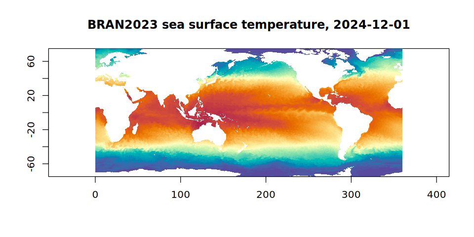

plot of chunk map

The cell centres come from the geotransform rather than from the coordinate variables: those are stored as 32-bit floats, so their spacing is not exactly regular, and image() draws a raster only from a grid that is. The land is blank because it was masked with the netCDF fill value. Latitude in BRAN runs from south to north, so the first row of this raster is the southernmost and its pixel height is positive.